---

---

Optimization is a non-negotiable step in building a high-performance semantic model. While lightning-fast query speeds depend on many variables, such as schema design, relationship complexity, and DAX efficiency, the lowest-hanging fruit is almost always model size. A leaner model isn’t just about saving space; it’s about agility and user experience.

In this post, we’ll share five practical tips that anyone, regardless of their skill level, can use to “slim down” their Power BI models today. Plus, a bonus pro-tip for those ready to take their optimization to the next level.

• Why model size matters
• Typical data flow in Power BI
• TIP 1: Disable auto date/time
• TIP 2: Only load the rows and columns that are necessary
• The Mechanics of Data Compression: Cardinality and Encoding
• TIP 3: Set the correct data type for columns
• TIP 4: Optimize datetime columns
• TIP 5: Optimize high-precision decimal columns
• TIP 6: Set “isAvailableInMdx” to false
• Conclusion

---

Why model size matters

A bloated semantic model is more than just a storage nuisance; it’s a performance anchor that drags down the entire lifecycle of your report. From the frustration of a slow development environment to the literal cost of cloud resources, “carrying extra weight” in your data has tangible consequences for both developers and end users.

• Longer Refresh Times: Every extra row or column forces the VertiPaq engine to work harder during processing. This extends the data refresh durations and keeps your data sources and data gateways busy for longer.
• Slower Query Performance: Large models require more CPU cycles to scan and aggregate data. This leads to those dreaded “spinning wheels” on your report pages, creating a laggy and frustrating experience for your users.
• Editing and Publishing Delays: Uploading a massive pbix file consumes significant bandwidth and time. When your model is oversized, even a minor DAX tweak can take minutes for the model to accept the change and later publish to the Service.
• Higher Memory Requirements: Fabric capacities have strict memory limits. A heavy model risks hitting these “ceilings,” which can lead to performance throttling or the costly need to upgrade to a higher capacity tier.
• Increased Data Transfer and Storage Costs: Cloud resources aren’t free, and moving large volumes of data across networks incurs egress fees.
• Frequent Failures and Retries: Bloated models are far more likely to trigger “Out of Memory” errors or timeouts during a refresh.
• Electricity Consumption and Carbon Emissions: Data processing requires significant server power. By optimizing your model, you reduce the energy needed to compute and store your data, thereby contributing to a lower carbon footprint.

Before delving into tips to reduce your model’s footprint, it is important to understand how data is processed and stored in Power BI, as well as the difference between a model’s offline and memory sizes.

Typical data flow in Power BI

In import mode models, the process begins when Power BI connects to a data source via Power Query to ingest data, perform necessary transformations, and clean it. Once processed, this data is passed to the VertiPaq storage engine, which encodes and compresses it. The VertiPaq engine is remarkably efficient, often achieving a compression ratio of up to 10x compared to the raw source data. The resulting footprint of the model when stored on a disk or within the Power BI Service is referred to as the offline size.

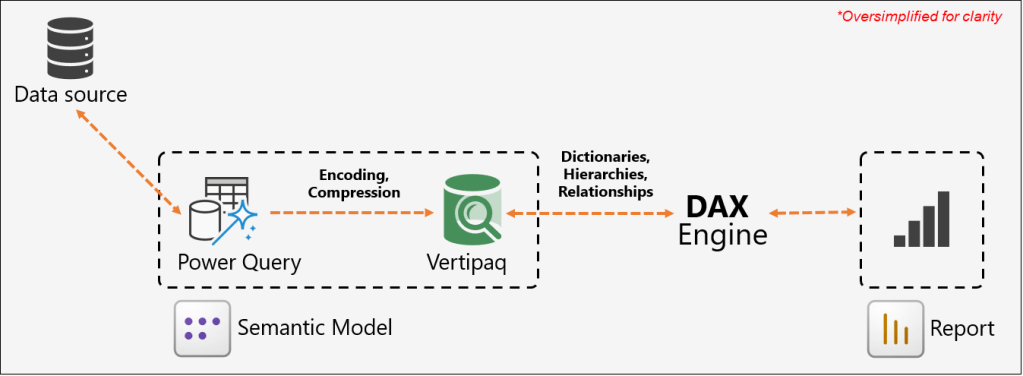
When a user opens a report, the visuals on the page generate queries that are sent to the DAX engine for evaluation. To resolve these queries and perform calculations, the engine must access the underlying data. To fulfill the data request, the VertiPaq engine loads the necessary columns into the system’s RAM. The VertiPaq engine must also allocate memory for dictionaries (maps of unique values), hierarchies, and relationships to make the data accessible and searchable. This total footprint in the system’s RAM is known as the memory size. The DAX engine then evaluates these queries against the loaded data and returns the results to the report, where the visuals are populated and displayed to the user.

The memory size is typically larger than the offline Size because your data needs “breathing room” to actually work. When the model is saved to disk, it is tightly packed and “asleep”. However, once you open a report, the VertiPaq engine must load the data into RAM and build active structures such as dictionaries, hierarchies, and relationship maps to make the data searchable. This matters because while the offline size determines your file storage, the memory size determines your actual performance. If the memory footprint is too large, it can lead to slower visuals, refresh failures, and “Out of Memory” errors as the engine runs out of space to perform its calculations.

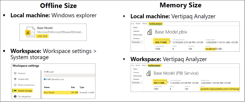
Determining Model Size: Offline vs. Memory

Finding the model’s offline size is straightforward. On a Windows machine, you can view the file size of your .pbix file just like any other file. In the Power BI Service, this size is visible within your workspace under Workspace settings > System storage.

However, identifying the memory size is a more technical process that requires an external tool called VertiPaq Analyzer. This tool scans the underlying storage structures to provide detailed statistics on the memory usage of each column and table. It can analyze models currently open in Power BI Desktop on your local machine, as well as published models hosted in a Power BI workspace via the XMLA endpoint. More on VertiPaq Analyzer later in the article.

To help you gauge the impact of your changes, we recommend using VertiPaq Analyzer to monitor your model’s memory size throughout the optimization process. By checking the statistics before and after each step, you can precisely assess the effectiveness of each tip and see exactly how much memory you are saving.

TIP 1: Disable auto date/time

When the Auto date/time setting is enabled, Power BI automatically creates a hidden table for each date column in your model to support basic time intelligence (such as Year, Quarter, Month, and Day hierarchies). While this sounds convenient, it is a major source of hidden “model bloat.” Keep in mind:

• They are invisible: These tables do not appear in the Fields pane, Model view, or Table view.
• They are restrictive: You cannot reference these hidden tables or their columns directly in DAX expressions, nor do they work when using Analyze in Excel.
• They multiply quickly: If you have ten different date columns across your model, Power BI creates ten separate hidden tables, significantly increasing your memory size.

Auto date/time tables can consume a significant amount of memory, increasing with each date column in your model. In large-scale semantic models, we have observed these hidden tables consuming up to 500 MB of memory. Because they are generated automatically for every date field, the bloat adds up quickly and silently. The fastest way to instantly shrink your model size and regain that memory is to disable the auto date/time settings and replace those redundant hidden tables with a single, optimized, and dedicated Date table.

Configuring Auto date/time

You have full control over this feature, and you can toggle it on or off at any time. It can be configured in two ways in Power BI Desktop:

• Go to File > Options and settings > Options.
• Under GLOBAL, select Data Load and uncheck Auto date/time for new files under Time intelligence. This option applies to all new Power BI Desktop files you create going forward.

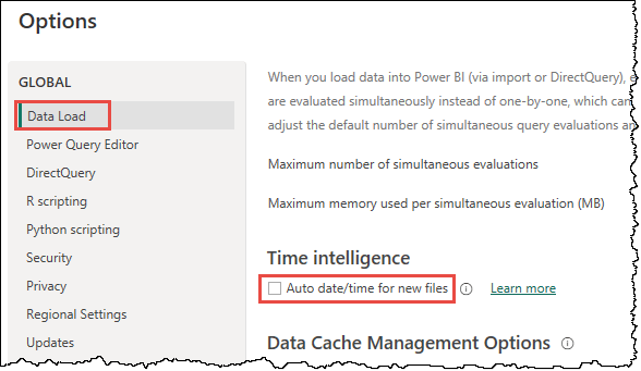
• Under CURRENT FILE, select Data Load and uncheck Auto date/time under Time intelligence. This option applies to the file you are currently working on.

ℹ️ Since auto date/time tables are permanently hidden from the Power BI Desktop UI, you might wonder how actually to see them or measure their memory consumption.

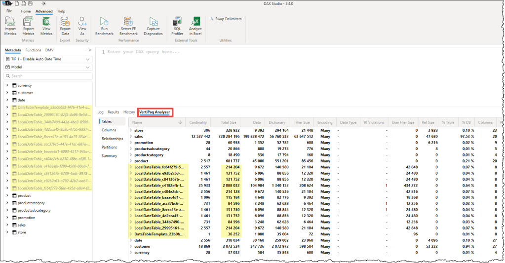
• View auto date/time tables: Connect your model to DAX Studio. Even though they are hidden in the Power BI Model View, these tables will appear in the DAX Studio metadata pane, typically named with a prefix like LocalDateTable_.
• Measure memory consumption: Use the VertiPaq Analyzer in DAX Studio. It will list every hidden date table individually, showing exactly how much memory each consumes. These small, convenient tables can collectively account for a surprising percentage of your total model size.

A recommended approach is to have an organization-wide standardized Date table that everyone can use in their semantic models. A highly effective way to do this is to provide a Power BI Template (.pbit) that includes a preconfigured date table as a starting point for every new semantic model. Alternatively, you can store the table definition as a TMDL or C# script in a centralized location, such as a Git repository or a SharePoint site, so everyone on your team and in your organization can use it. These approaches ensure that individual models remain lean and time intelligence calculations and date formats remain uniform across all reports.

You can also use the Bravo or C# scripts from the Tabular Editor team to create a date table in your model.

TIP 2: Only load the rows and columns that are necessary

Optimization begins with a simple rule: if it isn’t being used in a report, it shouldn’t be in your model. Every unnecessary row or column forces the VertiPaq engine to consume more memory for dictionaries and hierarchies, which inevitably slows down the performance. While it is easy to say you should only add the tables you need, it is less clear how to decide which rows and columns to cut.

Here are the key points to keep in mind when slimming down your model:

Only Load the Necessary Rows

Before importing data, ask yourself if the full history is truly required for your current business use case. If you are building a report specifically for “Actuals,” there is no reason to load “Forecast” or “Budget” data into the same model. You should filter your data at the source or in Power Query to include only the specific years, scenarios, or geographic regions required. Remember, it is much easier to add more data later than it is to manage a huge, sluggish model today.

Remove Columns That Are Not Required

Not all columns are created equal. Most of the columns fall into one of the following four categories:

• Keys (Primary/Foreign): These are essential for relationships, but if a key isn’t being used to connect tables, it should be removed.
• Qualitative & Quantitative Attributes: These are the descriptive labels (text) and values (numbers) used for filtering and calculations. These are the core of your model and should be kept.
• Descriptive Attributes: These provide extra details about a row but aren’t used for filtering. Only keep these if they are necessary for “drill-through” operations.
• Technical Attributes: These are metadata fields (like “Created Date” or “Record ID”) that have no business value. The application or database engine usually creates these columns. Unless needed for specific audit or drill-through purposes, these should be the first to go.

Where to focus your efforts: When applying this tip, your primary targets should always be your fact tables. Because fact tables contain the highest volume of rows, removing a single unused column there will have a much greater impact on memory than removing a column from a small dimension table. While maintaining clean dimension tables is good practice, the real optimization for model size happens in the fact data.

While this tip is straightforward in theory, it can be challenging to implement in a centralized or shared model. When multiple developers are building separate reports from a single semantic model, it becomes difficult for any one person to determine which columns or rows are truly “safe” to delete without combing through every connected report.

To solve this, you can use Measure Killer. Measure Killer is a third-party tool that scans all connected reports and identifies which columns are not used in any visuals or filters so that you can remove them with confidence.

ℹ️Unused Measures: While removing unused measures is a recommended practice, it is important to note that measures do not consume memory space. Deleting them won’t shrink your model size, but it is excellent for “model hygiene.” Removing clutter improves the user experience, especially when users are using perspectives to build their own visuals.

Before diving into the next tips, it is essential to understand the core techniques the VertiPaq engine uses to achieve such high levels of compression. Understanding these fundamentals is the secret to a high-performance model, as it allows you to structure your data so the engine can work at its maximum efficiency.

The Mechanics of Data Compression: Cardinality and Encoding

At the heart of the VertiPaq engine’s efficiency is a concept called cardinality. In simple terms, cardinality refers to the number of unique values in a column. For example, a “Gender” column has a very low cardinality (usually 2 or 3 unique values), while a “Transaction ID” column has a very high cardinality because each row is unique. Column cardinality is more significant for the model size than the total number of rows.

Cardinality is the primary driver of model size because of how the VertiPaq engine “encodes” or translates your data into a compressed format. The engine primarily uses two encoding methods to shrink your data:

• Hash Encoding (Dictionary Encoding): Used for text or high-cardinality data. The engine builds a dictionary of every unique value and assigns each a simple integer index. Instead of storing a long string like “Product_Name_XYZ” a million times, it stores the index “1.” If your cardinality is high, this dictionary becomes very large and consumes significant memory.
• Value Encoding: Used for numerical data. The engine uses mathematical logic to store numbers more efficiently, for example, by storing differences rather than the full numbers. This is the “gold standard” for performance because it requires no dictionary and allows the DAX engine to perform calculations directly on the encoded data.

By reducing cardinality, you directly shrink the size of these dictionaries and, in some cases, help the engine switch from hash encoding to the more efficient value encoding.

ℹ️The “hidden” processing phase: You may have noticed that when refreshing large tables, the Power BI loading wheel continues to spin long after the data transfer from the source has finished and the row counter has stopped updating. This occurs because the VertiPaq engine is working behind the scenes to determine the most efficient encoding strategy for your columns. During this phase, if the engine determines that a chosen strategy isn’t yielding the expected compression results or encounters a value it can’t encode with that strategy, it may discard the progress and restart the encoding process from scratch. This “hidden” optimization is what ensures your model remains as lean and fast as possible once the refresh completes.

VertiPaq Analyzer

VertiPaq Analyzer is a third-party tool and the only truly reliable way to measure the memory footprint of your semantic model. It provides a granular “under the hood” view of how the VertiPaq engine stores your data, allowing you to move beyond guesswork and make fact-based optimization decisions.

It exposes critical metrics for every column in your model, including:

• Cardinality: The number of unique values in a column.
• Total Size: The combined memory footprint of the column.
• Data & Dictionary Size: How much space is used by the values themselves and the unique value lookup table (the dictionary).
• Hierarchy & User Hierarchy Size: The memory used by MDX hierarchies and user-defined hierarchies.
• Relationship Size: The memory used by the internal indexes that map related columns between tables.
• Encoding: Which encoding method (Value or Hash) the engine chose for that specific column.
• Model Percentage (%DB / % Table): Exactly what portion of the model or table is being consumed by a single column.

VertiPaq Analyzer is conveniently built into both DAX Studio and Tabular Editor 3. It plays a central role in the optimization process; by running it before and after you apply your changes, you can see the immediate, measurable impact of your efforts on cardinality, encoding, and overall model size.

ℹ️Understanding “Many” encoding: You might notice in VertiPaq Analyzer that tables always list “Many” as the encoding type. This appears to be a design choice, as encoding applies to individual columns rather than tables.

A detailed description of encoding and compression techniques is out of the context of this article. You can find a great deal of detail about these online. The mentioned details are sufficient to understand their impact and the reason for our next tips to optimize your model size.

TIP 3: Set the correct data type for columns

The data type you choose is more than just a formatting preference; it is a direct instruction to the VertiPaq engine on how to store that data. Choosing the wrong type can force the engine into less efficient storage methods, unnecessarily inflating your model’s size.

Why data types matter

• Storage footprint: Different data types require different amounts of baseline memory. A “Fixed Decimal Number” (Currency) is often more efficient than a standard “Decimal Number.”
• Encoding strategy: The engine uses your data type to determine whether to use value encoding or hash encoding.
• Compression efficiency: The final storage size is directly determined by how well the encoding and RLE compress that specific data type.

“Data type impostors”

It is common to find columns that aren’t what they seem. These “impostors” are the silent killers of model performance. Keep an eye out for:

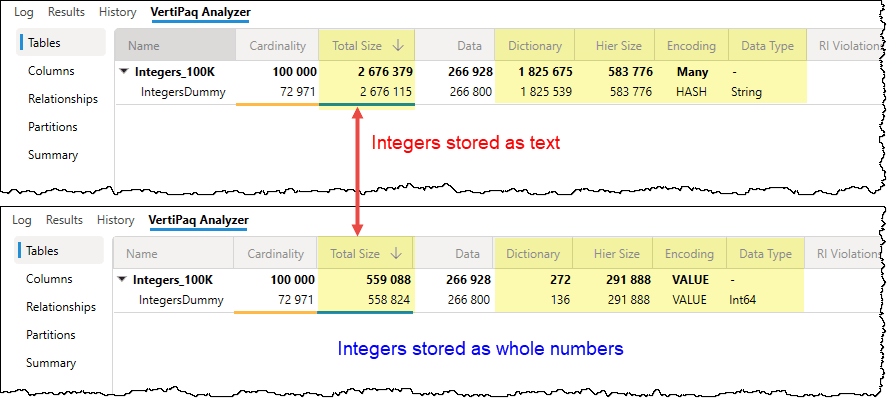
• Integers stored as Decimals or Text: If a column contains only whole numbers (e.g., an ID or Year), ensure it is set to Whole Number.
• Decimals stored as Text: This is the most expensive mistake, as it forces the engine to build a massive text-based dictionary for values that should be handled with simple math.

The following two tips stem from a single, critical question: What is the minimum level of granularity at which the data should be presented in the report? By determining the exact level of detail your users actually need, you can significantly reduce the volume of data the VertiPaq engine has to process. Defining this “grain” upfront is the most effective way to optimize your model.

TIP 4: Optimize datetime columns

The storage impact of a Date/Time column is directly tied to its cardinality (the number of unique values). The more precise your timestamps, the higher the cardinality, and the more memory the VertiPaq engine requires for dictionaries and encoding.

To reduce the size of these columns, you must set their precision to the minimum required for your business needs. Consider the math of cardinality:

• Date only: 10 years of date equals only about 3,653 unique values.
• Date + Time (to the second): 1 day of timestamp could potentially reach over 86,000 unique values.

Timestamp Unit	Cardinality
Hour	24
15 Minutes	96
5 Minutes	288
Minute	1,440
Second	86,400
Millisecond	86,400,000

This massive jump in uniqueness is what causes model bloat. Ask yourself: Do your users truly need to analyze data down to the second, or is the hour or minute sufficient?

How to optimize datetime columns

• Remove the time portion: If your analysis is daily (e.g., “Sales by Day”), change the data type to Date.
• Round to an acceptable granularity: If you must keep the time, consider rounding it to the nearest 15-minute, 30-minute, or 1-hour interval. This significantly lowers the number of unique values while still providing actionable insights.
• Split date and time into two columns: Instead of one “datetime” column, split it into two separate columns: one for Date and one for Time. Because each column is compressed independently, the VertiPaq engine can encode a small date dictionary and a small time dictionary (maximum 86,400 values for seconds), which is far more efficient than a single column containing every possible combination of the two.

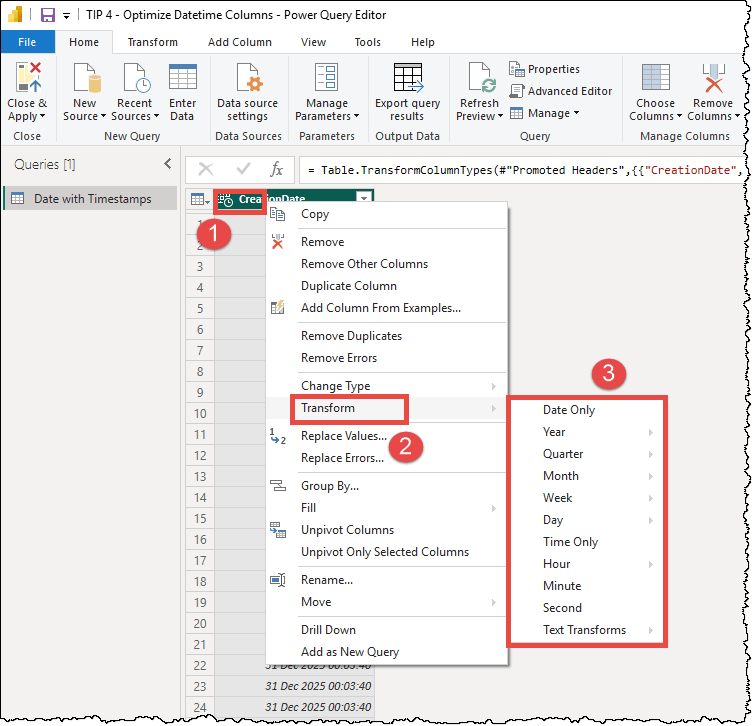
The Power Query editor offers built-in transformation options directly in the right-click menu of datetime columns. By selecting the Transform option, you can instantly extract the date, truncate the time to the start of the hour, or isolate specific components like the month or year, allowing you to reduce cardinality without writing a single line of code.

TIP 5: Optimize high-precision decimal columns

Just like with datetime columns, the storage “cost” of a decimal column is driven by its high cardinality. High-precision columns with five or more digits after the decimal point create a unique value for almost every row, preventing the VertiPaq engine from effectively using value encoding or RLE.

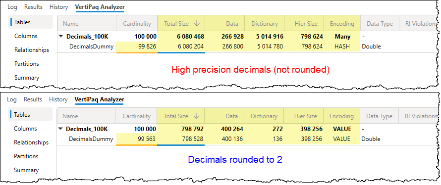
Ask yourself: Do your users truly need to see a value like 123.45678 in a report? In the vast majority of business cases, rounding to one or two decimal places (e.g., 123.5 or 123.46) provides the necessary insight while drastically reducing the number of unique values the engine must store.

How to optimize decimal columns

• Round to a fixed granularity: Rounding your values to two decimal places can collapse millions of unique floating-point values into a much smaller, highly compressible set.
• Split the integer and decimal parts into two columns: If you must maintain extreme precision for specific calculations, consider splitting the column into two: one for the whole number and one for the decimal remainder. This allows the engine to compress the whole numbers separately from the fractional parts.

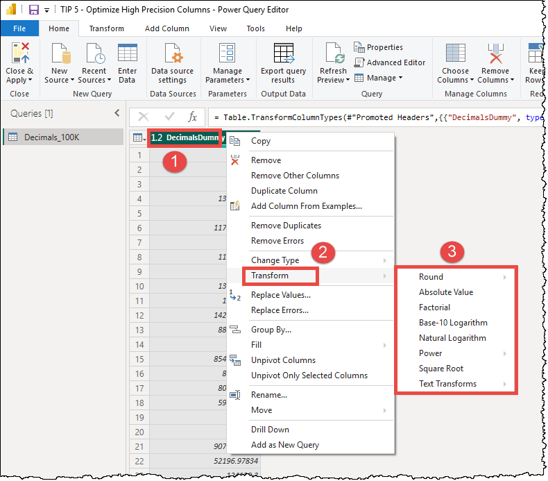
Similar to datetime columns, the Power Query editor offers built-in transformation options directly in the right-click menu of decimal columns. You can round up or down, keep only the absolute value, etc.

ℹ️While you can easily implement these optimizations: setting correct data types (Tip 3), reducing datetime cardinality (Tip 4), and rounding decimals (Tip 5) directly in Power Query, the most effective approach is to handle them at the data source. Whenever possible, apply these transformations within your data warehouse or database before the data even reaches Power BI. By fixing these issues at the source, you ensure that every colleague using those tables inherits the same optimized data. This strategy of moving the transformation to the source (Roche’s Maxim) not only keeps your semantic models lean but can also improve the efficiency of the data source itself.

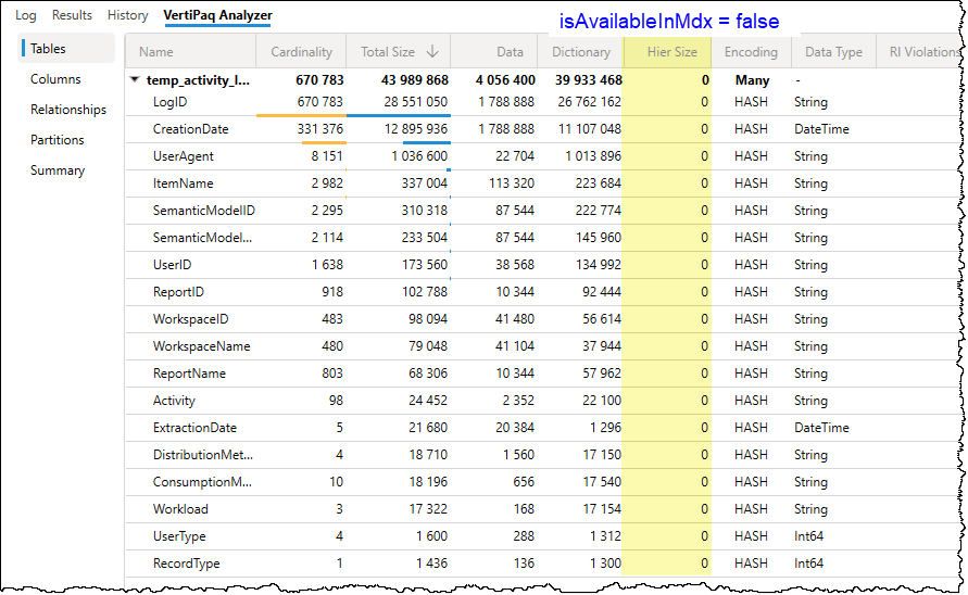
TIP 6: Set “isAvailableInMdx” to false

⚠️This is an advanced optimization tip. You should apply this tip only if you have a clear understanding of how your users interact with the model, as it specifically affects MDX-based tools such as “Analyze in Excel” and SQL Server Reporting Services (SSRS).

What is isAvailableInMDX

By default, this property is set to True for every column in your model. When true, the VertiPaq engine builds a special MDX attribute hierarchy for that column. This hierarchy allows Excel PivotTables to group and filter the data, but it also consumes additional memory and processing time during data refreshes.

The impact of changing isAvailableInMDX:

• Set to True (Default): The column is visible and usable in Excel PivotTables, but it increases the model’s memory footprint.

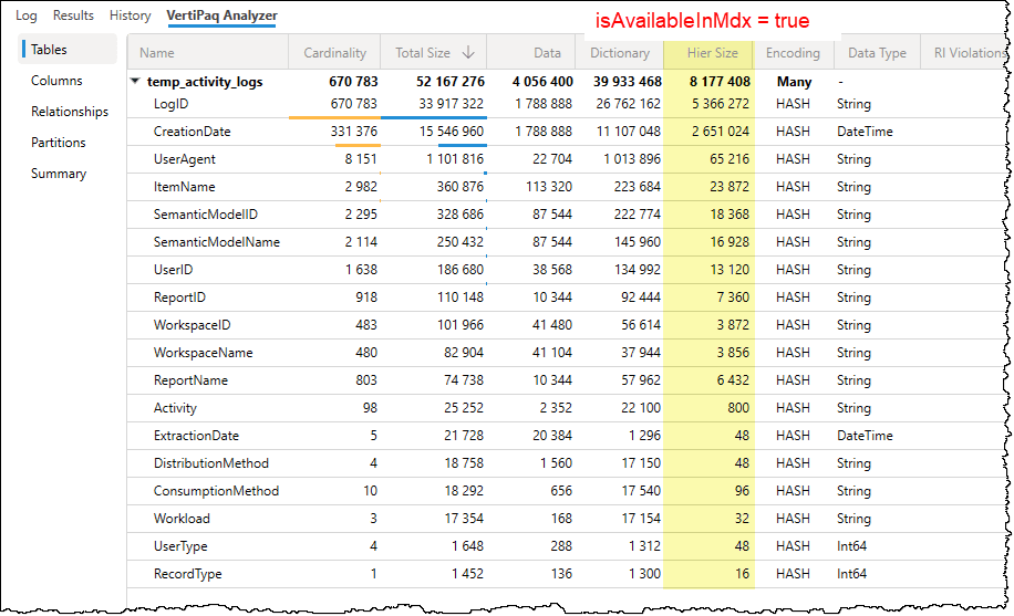
• Set to False: The MDX hierarchy is not built, reducing the model size and improving refresh speeds. However, that column will no longer be available for use in “Analyze in Excel” or other MDX-based clients.

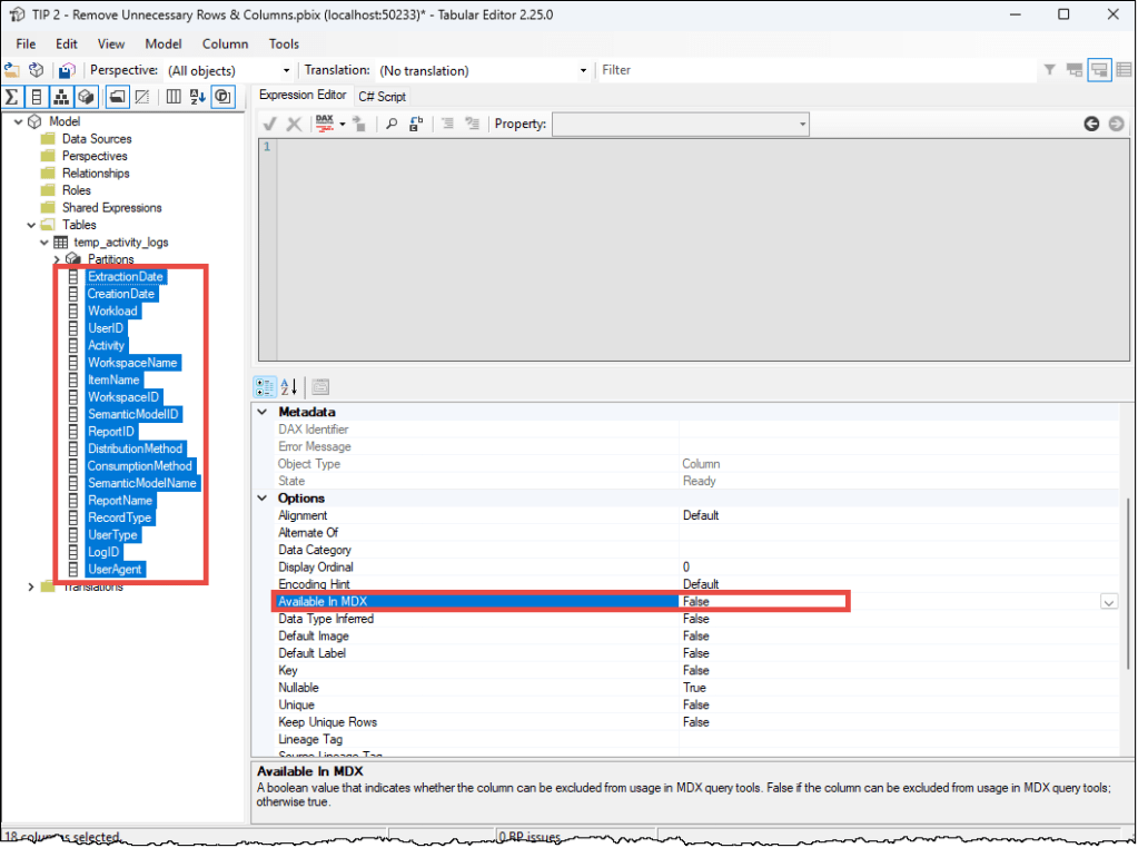
Power BI Desktop does not provide a native UI option for this property. To change it, you have two primary options:

• Tabular Editor: This is the fastest method. You can select multiple columns in Tabular Editor 2 or 3 and batch-set the isAvailableInMDX property to false. Alternatively, you can use a C# script.

• TMDL Scripts: In Power BI Desktop, you can use the TMDL (Tabular Model Definition Language) script to set column values to false manually. Note that since the default value of isAvailableInMDXis true, the property is hidden from the column’s TMDL definition until you manually define it as false, i.e., isAvailableInMdx: false

Recommendation: If you are certain your model will never be used in Excel, you can set it to false for all the columns in the model. Otherwise, disable it for technical columns, long description columns, key columns used in relationships, fact table columns, hidden columns, etc., that no one would ever realistically use in an Excel PivotTable. 

That’s all for now. There are some other tips to reduce model size, but these six are the easiest to implement and work in all scenarios.

Conclusion

Ultimately, a well-optimized model is about more than just a smaller file size; it’s about providing a seamless, lightning-fast experience for your end users. By mastering these six tips, you transition from simply building reports to designing professional-grade semantic models that are scalable, maintainable, and cost-effective.

In summary, optimizing a semantic model is a strategic process of reducing “noise” to let the VertiPaq engine shine.